Next: Fit procedure
Up: Fitting of histograms
Previous: Fitting of histograms
The basic peak shape is assumed to be a sum of asymmetric
Gaussian with widths  depending on the particle type
(index
depending on the particle type
(index  ) and track length (number of points
  ):
):
 |
(1) |
The basic parameter setting the width is  which is fitted
for all bins. The dependence on path-length is assumed to be
which is fitted
for all bins. The dependence on path-length is assumed to be
 . The exact dependence on is not a real concern, since
the number-of-points distribution is quite strongly peaked in each
phase space bin. The dependence of the width on the
. The exact dependence on is not a real concern, since
the number-of-points distribution is quite strongly peaked in each
phase space bin. The dependence of the width on the  peak
position
peak
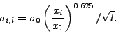
position  is parameterised as a power law with power 0.625.
This number was extracted from simultaneous fits to
is parameterised as a power law with power 0.625.
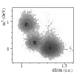
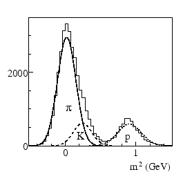
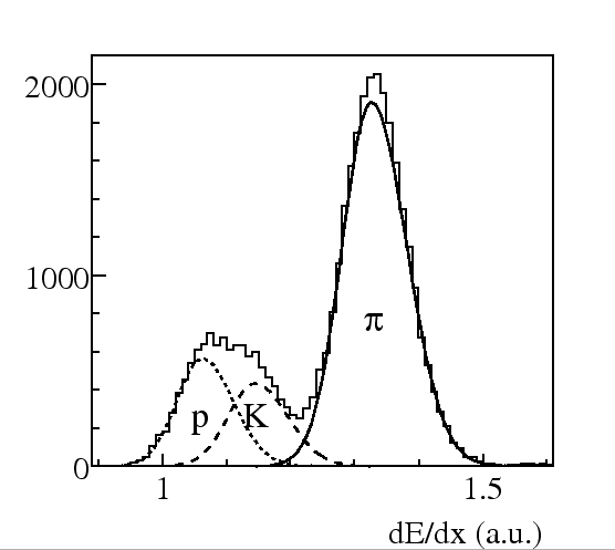
This number was extracted from simultaneous fits to  from TOF and
from the TPC, as illustrated in Figs 1
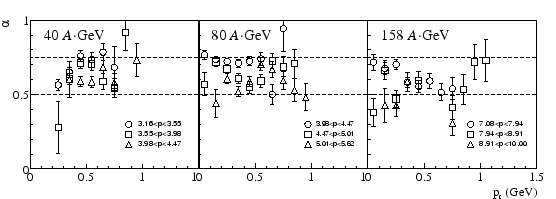
[2]. Fig 2 shows the result of
the two-dimensional fits for the higher beam energies (40, 80 and 158
GeV). The points clearly cluster at values of
from TOF and
from the TPC, as illustrated in Figs 1
[2]. Fig 2 shows the result of
the two-dimensional fits for the higher beam energies (40, 80 and 158
GeV). The points clearly cluster at values of  slightly above
0.5, but significantly below unity. The value 0.625 was takena s a
certal value and the sensitivity to this parameter was investigated
and found to be small (a few per cent at maximum, for 40
slightly above
0.5, but significantly below unity. The value 0.625 was takena s a
certal value and the sensitivity to this parameter was investigated
and found to be small (a few per cent at maximum, for 40
 and
above).
and
above).
Figure 2:
Value of the scaling parameter
for the width of the
peaks as a function of the position, as determined in
different bins of total momentum and  . The different panels
show results at the three different beam energies. The dashed lines are at
. The different panels
show results at the three different beam energies. The dashed lines are at
 .
.
 |
The Gaussian peaks are allowed to be asymmetric to reflect the
remainder of the tail of the Landau-distribution which is still
present in our truncated mean measure of . The total formula
for fitting the distribution is then
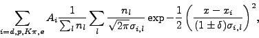 |
(2) |
where  are the amplitudes (yields) of each peak. The
  are
numbers of tracks with a certain length, so the second sum is simply
the weighted average of the line-shape from the different
track-lengths in the sample.
are
numbers of tracks with a certain length, so the second sum is simply
the weighted average of the line-shape from the different
track-lengths in the sample.
The fit function is evaluated in the T49SumGaus class.
Next: Fit procedure
Up: Fitting of histograms
Previous: Fitting of histograms
Marco van Leeuwen
2009-01-14